| Month | Occupancy-Days | Electrical Costs |
|---|---|---|
| January | 1,736 | 4,127 |
| February | 1,904 | 4,207 |
| March | 2,356 | 5,083 |
| April | 960 | 2,857 |
| May | 360 | 1,871 |
| June | 744 | 2,696 |
| July | 2,108 | 4,670 |
| August | 2,406 | 5,148 |
| September | 840 | 2,691 |
| October | 124 | 1,588 |
| November | 720 | 2,454 |
| December | 1,364 | 3,529 |
Required:
- Using the high-low method, estimate the fixed cost of electricity per month and the variable cost of electricity per occupancy-day. (Do not round your intermediate calculations. Round your Variable cost answer to 2 decimal places and Fixed cost element answer to nearest whole dollar amount.)
Variable cost of electricity 1.56 per occupancy-day Fixed cost of electricity 1,395 per month - What other factors in addition to occupancy-days are likely to affect the variation in electrical costs from month to month? (You may select more than one answer. Single click the box with the question mark to produce a check mark for a correct answer and double click the box with the question mark to empty the box for a wrong answer. Any boxes left with a question mark will be automatically graded as incorrect.)
Explanation
1.
\(\begin{align*}Occupancy-Days Electrical Costs High activity level (August) 2,406 5,148 Low activity level (October) 124 1,588 Change 2,282 3,560
\text{Variable cost} &= \text{Change in cost} ÷ \text{Change in activity} \\[6pt] &= $3{,}560 ÷ 2{,}282 \ \text{occupancy-days} \\[6pt] &= $1.56 \ \text{per occupancy-day}
\end{align*}\)2.Total cost (August) 5,148 Variable cost element ($1.56 per occupancy-day × 2,406 occupancy-days) 3,753 Fixed cost element 1,395
Electrical costs may reflect seasonal factors other than just the variation in occupancy days. For example, common areas such as the reception area must be lighted for longer periods during the winter than in the summer. This will result in seasonal fluctuations in the fixed electrical costs.Additionally, fixed costs will be affected by the number of days in a month. In other words, costs like the costs of lighting common areas are variable with respect to the number of days in the month, but are fixed with respect to how many rooms are occupied during the month.
Other, less systematic, factors may also affect electrical costs such as the frugality of individual guests. Some guests will turn off lights when they leave a room. Others will not.
| Month | Units Shipped | Total Shipping Expense |
|---|---|---|
| January | 3 | 2,400 |
| February | 6 | 2,900 |
| March | 4 | 2,300 |
| April | 5 | 2,600 |
| May | 7 | 2,900 |
| June | 8 | 3,900 |
| July | 1 | 1,800 |
Required:
1-a. Prepare a scattergraph using the data given above. Plot cost on the vertical axis and activity on the horizontal axis.
Instructions:
- On the graph below, use the point tool (January) to plot units shipped on the horizontal axis and the shipping expense on the vertical axis.
- Repeat the same process for the plotter tools (February to July).
- To enter exact coordinates, click on the point and enter the values of x and y.
- To remove a point from the graph, click on the point and select delete option.
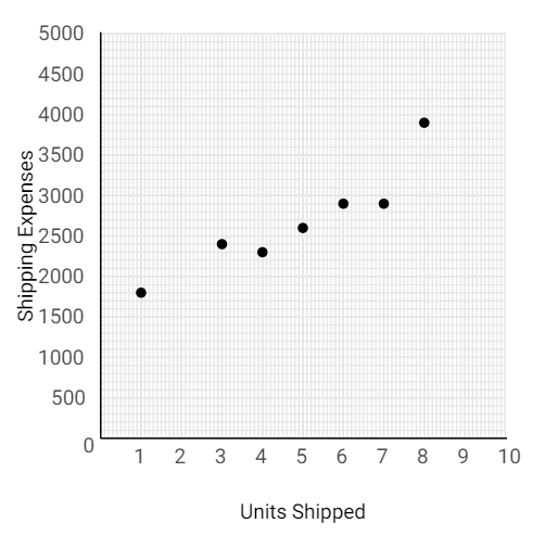
1-b. Is there an approximately linear relationship between shipping expense and the number of units shipped?
Explanation
1-b.
Yes, there is an approximately linear relationship between the number of units shipped and the total shipping expense.
| Month | Units Shipped | Total Shipping Expense |
|---|---|---|
| January | 3 | 2,400 |
| February | 6 | 2,900 |
| March | 4 | 2,300 |
| April | 5 | 2,600 |
| May | 7 | 2,900 |
| June | 8 | 3,900 |
| July | 1 | 1,800 |
Required:
2. Using the high-low method, estimate the cost formula for shipping expense.
| Variable shipping expense | 300 | per unit |
| Fixed shipping expense | 1,500 | per month |
Explanation
2.
The high-low estimates and cost formula are computed as follows:
| Units Shipped | Shipping Expense | |
|---|---|---|
| High activity level (June) | 8 | 3,900 |
| Low activity level (July) | 1 | 1,800 |
| Change | 7 | 2,100 |
Variable cost element:
\(\begin{align*}\frac{\text{Change in expense}}{\text{Change in activity}} = \frac{$2{,}100}{7 \ \text{units}} = $300 \ \text{per unit}
\end{align*}\)
Fixed cost element:
| Shipping expense at high activity level | 3,900 |
| Less variable cost element ($300 per unit × 8 units) | 2,400 |
| Total fixed cost | 1,500 |
The cost formula is $1,500 per month plus $300 per unit shipped or
\(Y = $1{,}500 + $300X \),where X is the number of units shipped.
| Month | Units Shipped | Total Shipping Expense |
|---|---|---|
| January | 3 | 2,400 |
| February | 6 | 2,900 |
| March | 4 | 2,300 |
| April | 5 | 2,600 |
| May | 7 | 2,900 |
| June | 8 | 3,900 |
| July | 1 | 1,800 |
4. What factors, other than the number of units shipped, are likely to affect the company’s shipping expense? (You may select more than one answer. Single click the box with the question mark to produce a check mark for a correct answer and double click the box with the question mark to empty the box for a wrong answer. Any boxes left with a question mark will be automatically graded as incorrect.)
Explanation
4.
The cost of shipping units is likely to depend on the weight and volume of the units shipped and the distance traveled as well as on the number of units shipped. In addition, higher cost shipping might be necessary to meet a deadline.
| Quarter | Tons Mined | Direct Labor-Hours | Utilities Cost |
|---|---|---|---|
| Year 1: | |||
| First | 25,000 | 6,000 | 60,000 |
| Second | 17,000 | 4,000 | 55,000 |
| Third | 30,000 | 5,000 | 70,000 |
| Fourth | 22,000 | 7,000 | 85,000 |
| Year 2: | |||
| First | 28,000 | 12,000 | 118,000 |
| Second | 35,000 | 12,000 | 123,000 |
| Third | 40,000 | 10,000 | 95,000 |
| Fourth | 38,000 | 13,000 | 132,000 |
Required:
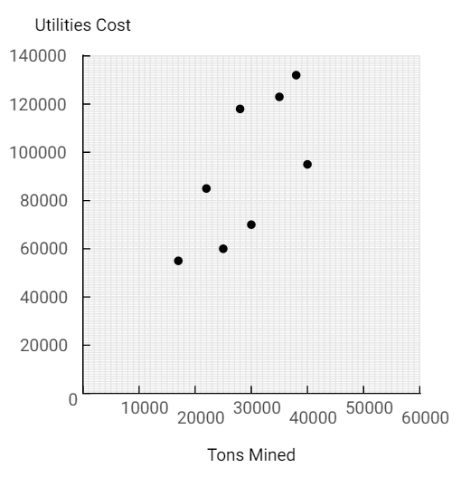
1-a. Using tons mined as the independent variable, prepare a scattergraph that plots tons mined on the horizontal axis and utilities cost on the vertical axis.
Instructions:
- On the graph below, use the point tool (Year 1-1st quarter) to plot tons mined on the horizontal axis and utilities cost on the Vertical axis.
- Repeat the same process for the plotter tools (Year 1-2nd quarter to Year 2-4th quarter).
- To enter exact coordinates, click on the point and enter the values of x and y.
- To remove a point from the graph, click on the point and select delete option.
1-b. Using the least-squares regression method, estimate the variable utilities cost per ton mined and the total fixed utilities cost per quarter. Express these estimates in the form Y = a + bX. (Round the Variable cost per unit to 2 decimal places and Fixed Cost to the nearest whole dollar amount.)
| Y = | 16,742 | + | 2.57 | X |
|---|
Explanation
1-a. & 1-b.
The cost formula, in the form Y = a + bX, using tons mined as the activity base is $16,742 per quarter plus $2.57 per ton mined, or
\(Y = $16{,}742 + $2.57X\) Note that the \(R^2\) is approximately 0.48, which means that only 48% of the variation in utility costs is explained by the number of tons mined.| Quarter | Tons Mined | Direct Labor-Hours | Utilities Cost |
|---|---|---|---|
| Year 1: | |||
| First | 25,000 | 6,000 | 60,000 |
| Second | 17,000 | 4,000 | 55,000 |
| Third | 30,000 | 5,000 | 70,000 |
| Fourth | 22,000 | 7,000 | 85,000 |
| Year 2: | |||
| First | 28,000 | 12,000 | 118,000 |
| Second | 35,000 | 12,000 | 123,000 |
| Third | 40,000 | 10,000 | 95,000 |
| Fourth | 38,000 | 13,000 | 132,000 |
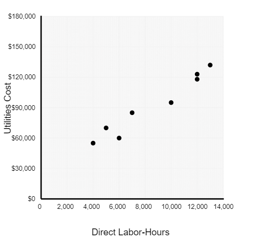
2-a. Using direct labor-hours as the independent variable, prepare a scattergraph that plots direct labor-hours on the horizontal axis and utilities cost on the vertical axis.
Instructions:
- On the graph below, use the point tool (Year 1-1st quarter) to plot direct labor-hours on the horizontal axis and utilities cost on the Vertical axis.
- Repeat the same process for the plotter tools (Year 1-2nd quarter to Year 2-4th quarter).
- To enter exact coordinates, click on the point and enter the values of x and y.
- To remove a point from the graph, click on the point and select delete option.
2-b. Using the least-squares regression method, estimate the variable utilities cost per direct labor-hour and the total fixed utilities cost per quarter. Express these estimates in the form Y = a + bX. (Round the Variable cost to 2 decimal places and Fixed Cost to the nearest whole dollar amount.)
| Y = | 21,802 | + | 8.17 | X |
|---|
Explanation
2-a. & 2-b.
The cost formula, in the form Y = a + bX, using direct labor-hours as the activity base is $21,802 per quarter plus $8.17 per direct labor-hour, or:
\(Y = $21{,}802 + $8.17X\) Note that the \(R^2\) is approximately 0.95, which means that 95% of the variation in utility costs is explained by direct labor-hours. This is a very high \(R^2\) which is an indication of a very good fit.| Quarter | Tons Mined | Direct Labor-Hours | Utilities Cost |
|---|---|---|---|
| Year 1: | |||
| First | 25,000 | 6,000 | 60,000 |
| Second | 17,000 | 4,000 | 55,000 |
| Third | 30,000 | 5,000 | 70,000 |
| Fourth | 22,000 | 7,000 | 85,000 |
| Year 2: | |||
| First | 28,000 | 12,000 | 118,000 |
| Second | 35,000 | 12,000 | 123,000 |
| Third | 40,000 | 10,000 | 95,000 |
| Fourth | 38,000 | 13,000 | 132,000 |
3. Would you recommend that the company use tons mined or direct labor-hours as a base for planning utilities cost?
Explanation
3.
The company should probably use direct labor-hours as the activity base, since the fit of the regression line to the data is much tighter than it is with tons mined. The \(R^2\) for the regression using direct labor-hours as the activity base is twice as large as for the regression using tons mined as the activity base. However, managers should look more closely at the costs and try to determine why utilities costs are more closely tied to direct labor-hours than to the number of tons mined.